
Credit Card Fraud Detector
Credit card fraud detector using supervised machine learning models.
● Abstract
The task of fraud detection is not an easy issue to solve, taking into account the multiple modalities and rapid evolution that this issue has currently had. Different supervised learning techniques are proposed since they use the assumption that fraudulent patterns can be learned from an analysis of past transactions. Within the proposed techniques, it will be seen that a better prediction is achieved with a neural network model using oversampled data and weighing the minority class.
● Introduction
Credit cards are part of the global commercial growth of the economies of emerging and developed countries through their traditional and online channels with the world. For this reason, it is important for credit card companies to be able to recognize fraudulent credit card transactions so that customers are not charged for items they did not purchase. Being such an important problem for the current economy, there is much research on it with different points of view. The most common are supervised techniques and within them models of neural networks, decision trees, support vector machines, among others, are used. For the use of supervised techniques, it is necessary to have data from past transactions, which must have been labeled according to whether the transaction was genuine (that is, it was carried out by the cardholder) or if it was fraudulent (that is, it was carried out by a scammer). These labels are usually known in hindsight, either because a customer complained or because they are the result of an investigation by the credit card company. With this information, the objective of this research is to design a model that can be used by companies capable of predicting the probability that a new transaction is fraud or not.
● Materials and methods
To solve the proposed problem, a database containing transactions made with credit cards in September 2013 by European cardholders will be used. This dataset presents the transactions that occurred in two days, where we have 492 frauds out of 284,807 transactions. The dataset is highly unbalanced, with the positive fraud class accounting for 0.172% of all transactions. The dataset contains numeric input variables that are the result of a principal component analysis (PCA) transformation, the only features that have not been transformed with PCA are time, class, and dollar amount in euros.
a. Proposed workflow
Below is a flowchart that indicates the different steps that were followed and within each one the different methodologies applied are detailed.
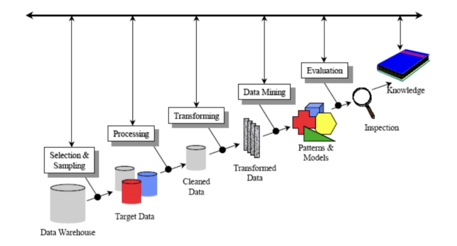
KDD aplicate
- Selection and Sample: As mentioned above, an already created dataset with 2-day transaction information was used.
- Processing: The dataset used did not have missing or duplicate data since it was previously processed with PCA.
- Transformation: in this stage, the Amount and Time columns were normalized using logarithmic and sinusoidal mapping functions, respectively. These features were chosen to maintain data continuity.
- Data Mining: The tools finally chosen to solve the problem were: neural networks with different architectures - linear regression - decision trees.
- Evaluation and Analysis: Finally, in this stage, the results obtained with the different models were compared.
b. Dataset split
Before starting with the training or with the preprocessing of the data, the data of the original dataset was divided into 3 groups for the training, validation and test stages. Since the data available is the result of 2-day transactions, for the third set, data belonging to 2 days is chosen to consider the temporary variable. For the division into training data and validation data, it was simply divided into data corresponding to the first day and data corresponding to the second day.
c. Balance of classes
The imbalance problem was addressed in 2 stages. In the first place, only those data that were within a radius defined as the maximum distance from the center of the distribution of fraudulent data to the furthest data were selected. That is to say, that transaction that does not belong to the radius zone is considered as “not fraud”. In a second stage, oversampling and undersampling algorithms were applied to the data obtained from the previous stage. This was done to compare the results obtained with one or the other. An algorithm was used that allows oversampling the minority class, in our case the fraud class. The algorithm used was the “SMOTE” algorithm, which basically consists of generating, from a sample x_i, a new sample x_{new} considering the k nearest neighbors. Then one of the nearest neighbors x_{zi} is chosen and the new sample is generated by interpolation:
x_{new} = x_i + \lambda x (x_{zi} - x_i)
Where \lambda is a random number in the range [0,1]. This interpolation creates a new sample on the line between x_i and x_{zi}. For the subsampling of the majority class, in our case the non-fraud class, the “NearMiss” algorithm was used. This algorithm can be divided into 2 steps. First, a nearest neighbor is used to make a shortlist of samples from the majority class. Then, the sample with the largest average distance to the k nearest neighbors is selected.
d. Choice of models
For the classification, 3 different models recommended in previous works were chosen:
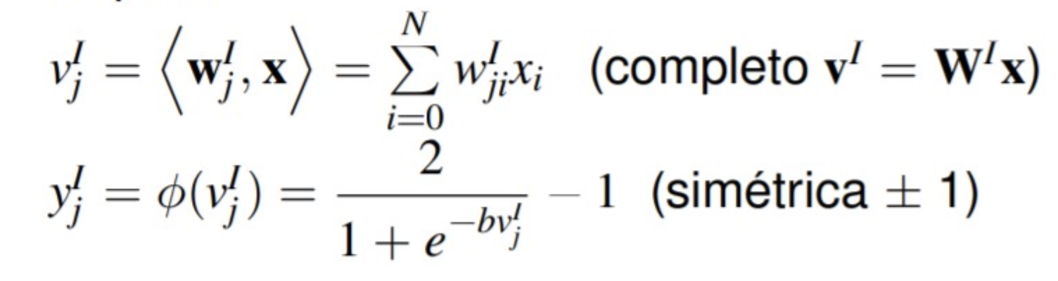
i) Neural networks: The artificial neural network (ANN) is a mathematical model inspired by the biological behavior of neurons and how they are organized to form the structure of the brain. Neural networks try to learn through repeated trials how to better organize themselves in order to maximize prediction.
Where the calculation of the outputs in each layer is:
• Layer I:
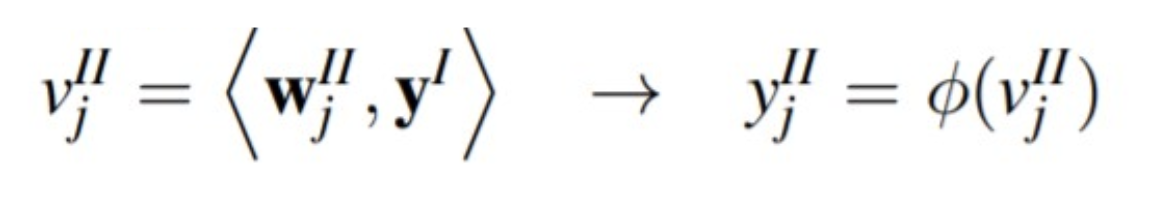
• Layer II:
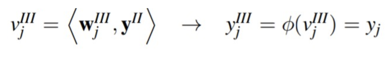
• Layer III:
ii) Logistic Regression: The output variable in a logistic regression model is qualitative, either 0 or 1 in the binary case. Therefore, a line cannot be made to associate the output with a data set. What is done then is to transform the qualitative output variable with a logistic operator. This mathematical operator tries to convert the variable to 0 or 1 , with a probability, that is, the probability of being from group 0 or from group 1.
For a data set with input Rn, we must obtain the unknown variables β, from the following function
y = \frac{1}{1 + e^{-1 ( \beta_0 + \beta_1 x_1 + \dots + \beta_n x_n)}}
This functional form is known as a simple perceptron.
iii) Decision trees: Random forest is a classifier consisting of a structured tree collection of classifiers {h(x, Θk), k = 1…} where {Θk} are independent and identically distributed. Also, each tree returns a voting unit for the most popular class at input x. There are several alternatives to find the purest and most homogeneous node possible, but the most used are the gini index and cross-entropy:
a. Gini index: It is considered a measure of purity of the node, its measure value ranges between (0) and (1) in such a way that values close to zero indicate purity of the node and close to one impurity; is a measure of the total variance of the kth constructed classes of the set.
b. Crossed Entropy: It is another way to quantify the disorder of a system. In the case of nodes, disorder corresponds to impurity. If a node is pure, containing only observations of one class, its entropy is zero. On the contrary, if the frequency of each class is the same, the entropy value reaches the maximum value of 1.
e. Evaluation measures
The objective of this stage is to evaluate the performance, weaknesses and strengths of the probabilistic models. To do this, a metric is used to select the probabilistic model that predicts the best results based on criteria such as accuracy, precision, recall.
Accuracy: Accuracy is an indicator that evaluates the ability of the model to correctly classify positive and negative cases into categories.
Accuracy = VP + VNVP + VN + FP + FN
Precision: Precision is the average probability of retrieving relevant information. It is a measure of accuracy or quality; high precision means that an algorithm returned substantially more relevant results than irrelevant ones.
Precision = VPVP + FP
Recall: It is the average probability of complete retrieval, here we take an average of several retrieval queries, while a high Recall means that an algorithm returned most of the relevant results.
Recall = VPVP + FN
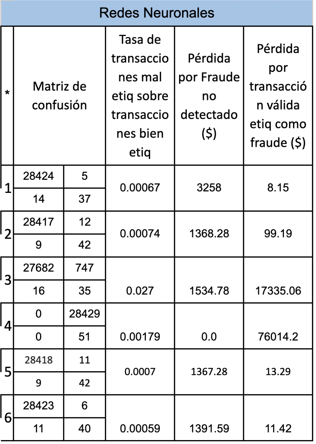
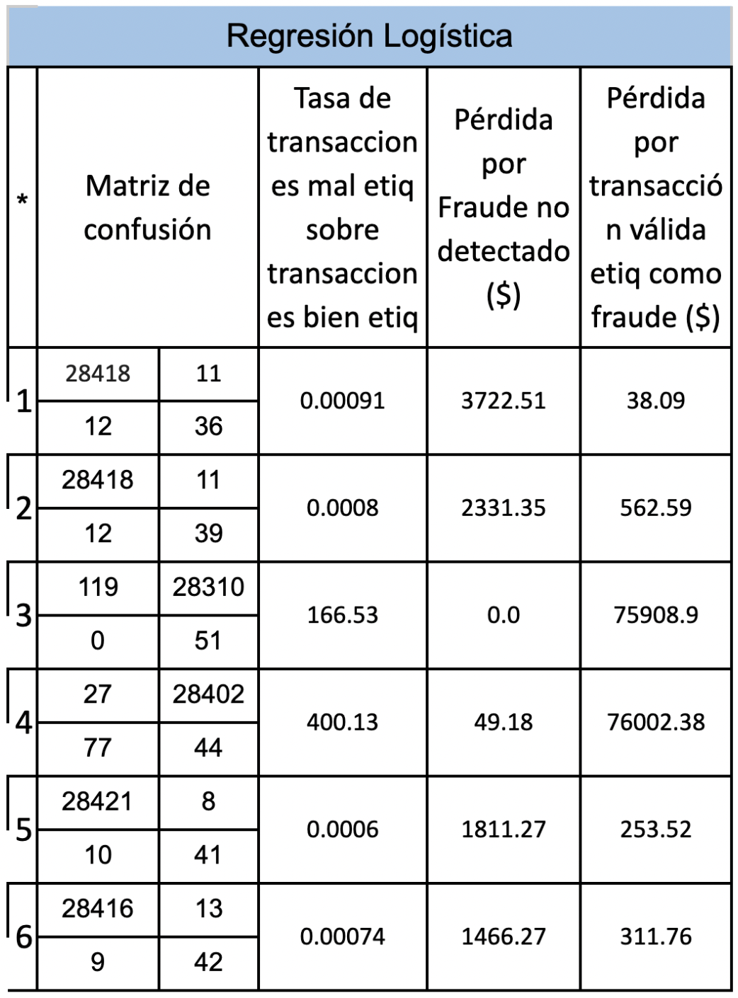
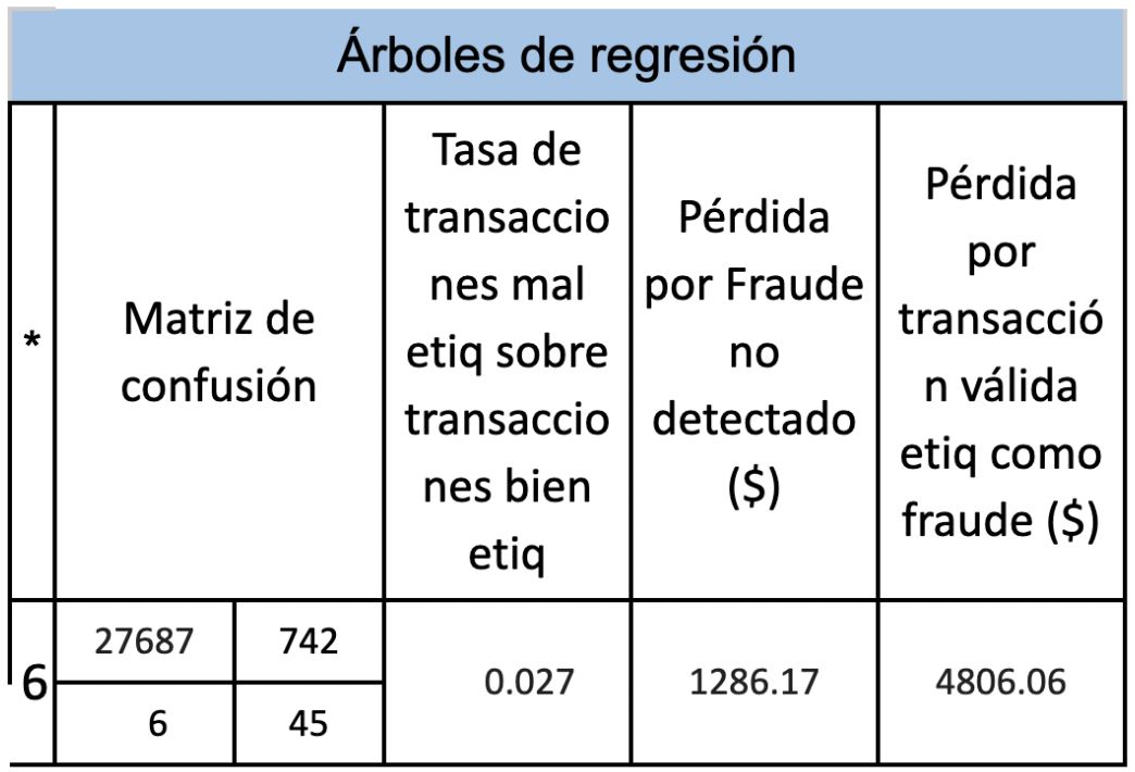
● Results
Next, 3 tables will be presented with the objective of comparing the different results according to the model and in turn according to whether oversampling or undersampling was carried out and if a weight factor was added to consider that an error in the prediction of fraud has an importance. greater than an error in the prediction of non-frauds. Where in * we have: 1 = data with nothing without weight 2 = data with nothing with weight 3 = unweighted undersampled data 4 = data subsampled with weight 5 = oversampled data without weight 6 = oversampled data with weight
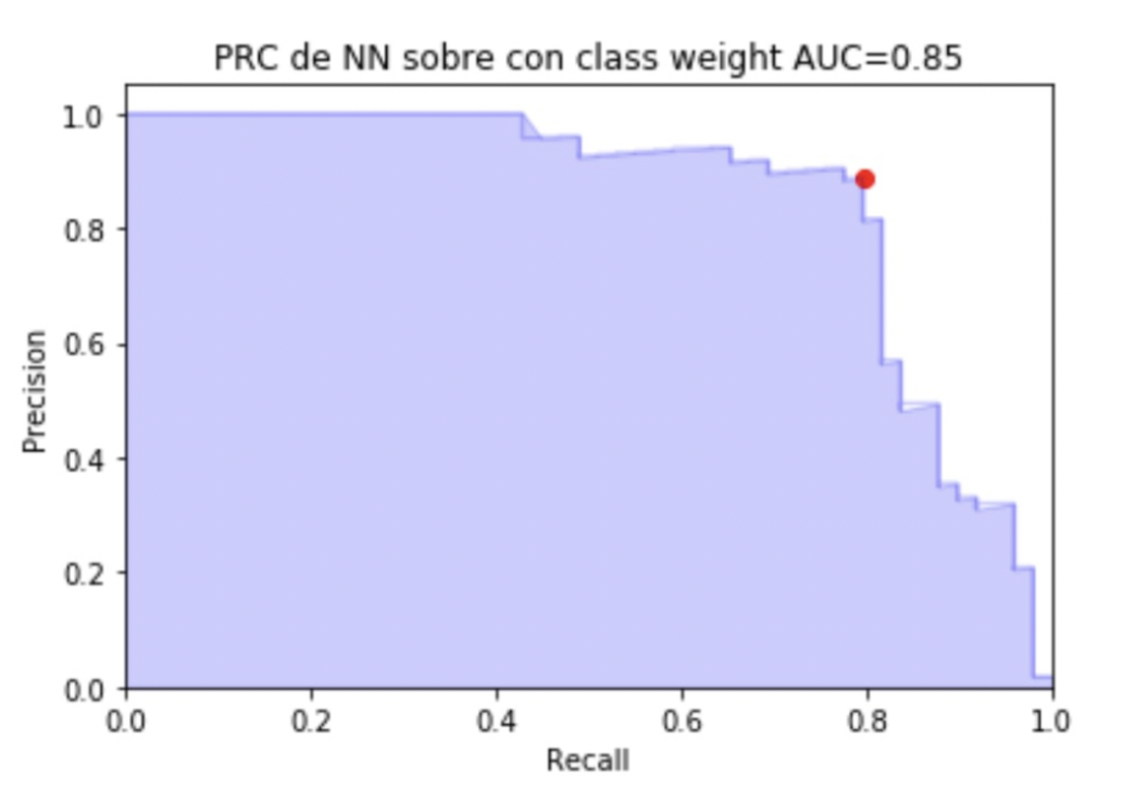
● Conclusions
Based on the results presented above, we can conclude that of the 3 models proposed regression trees is the one that requires less data preprocessing and the results are acceptable, the Logistic Regression model obtains its best result when the data is oversampled and when a weight is added to the minority class, and finally neural networks perform better when the data is oversampled and a weight is added to the minority class.